SQL Join → Postgres
One line: pull two CSV files in parallel, JOIN them inside a single SQL Transform, and write the joined rows into a Postgres table — all with four nodes and no Python.
This walkthrough builds a complete, working pipeline against a real Postgres database. Reading time 10 minutes; running time on the demo dataset is under 2 seconds.
By the end you will know how to:
- Wire two CSV sources into the same SQL Transform
- Use input ports so the SQL query can reference the sources by
table-style aliases (
customers,orders) - Configure the Postgres Target with structured fields the UI can validate
- Run the pipeline and verify the result on Postgres
Files
Download these into a local folder (the example below uses
/tmp/tutorials/sql-join/ but any absolute path on the same machine
where Odara runs works):
- customers.csv — 20 customers (id, name, email, country, signup_date)
- orders.csv — 60 orders (order_id, customer_id, product, quantity, total_amount, order_date)
The two files share customer_id, which is the JOIN key.
You'll also need a Postgres database you can write to. Anything works
— a local docker run postgres, an Aiven/Neon free tier, RDS, etc.
1. The shape of the pipeline
Four nodes in a Y-shape: two CSV sources feed into one SQL Transform, which feeds into one Postgres Target.
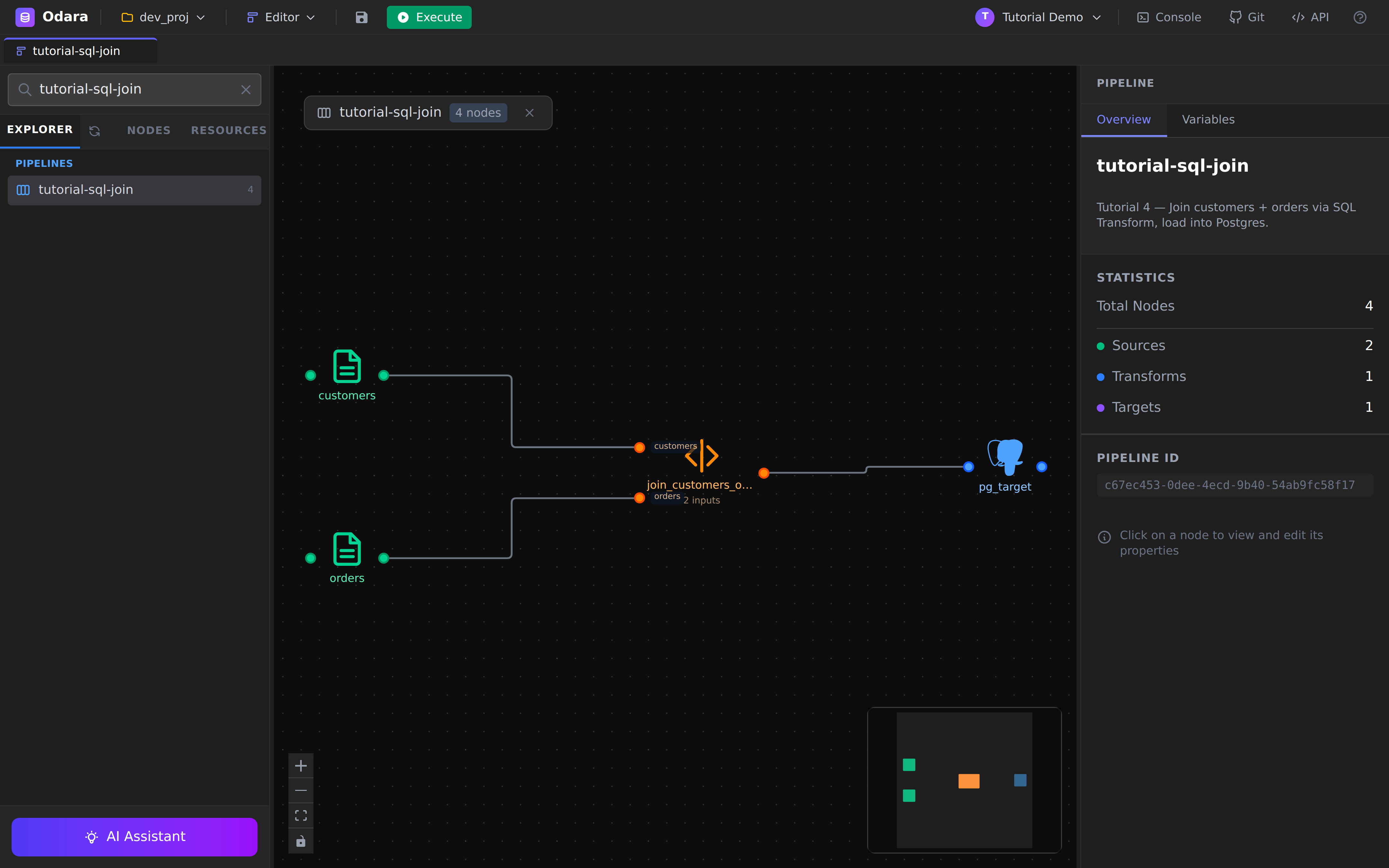
The right-hand Pipeline panel summarises what's on the canvas:
Total Nodes: 4, Sources: 2, Transforms: 1, Targets: 1. The
STATISTICS block is a quick sanity check that the canvas matches
what you intended before you hit Execute.
Notice the two small labels on the SQL Transform's input edges —
customers and orders. Those aren't decorative; they're
input port names and they become the table names the SQL
query joins on. We'll come back to this in §4.
2. CSV source — customers
Click the customers node on the canvas. The Properties panel on the right shows its configuration.
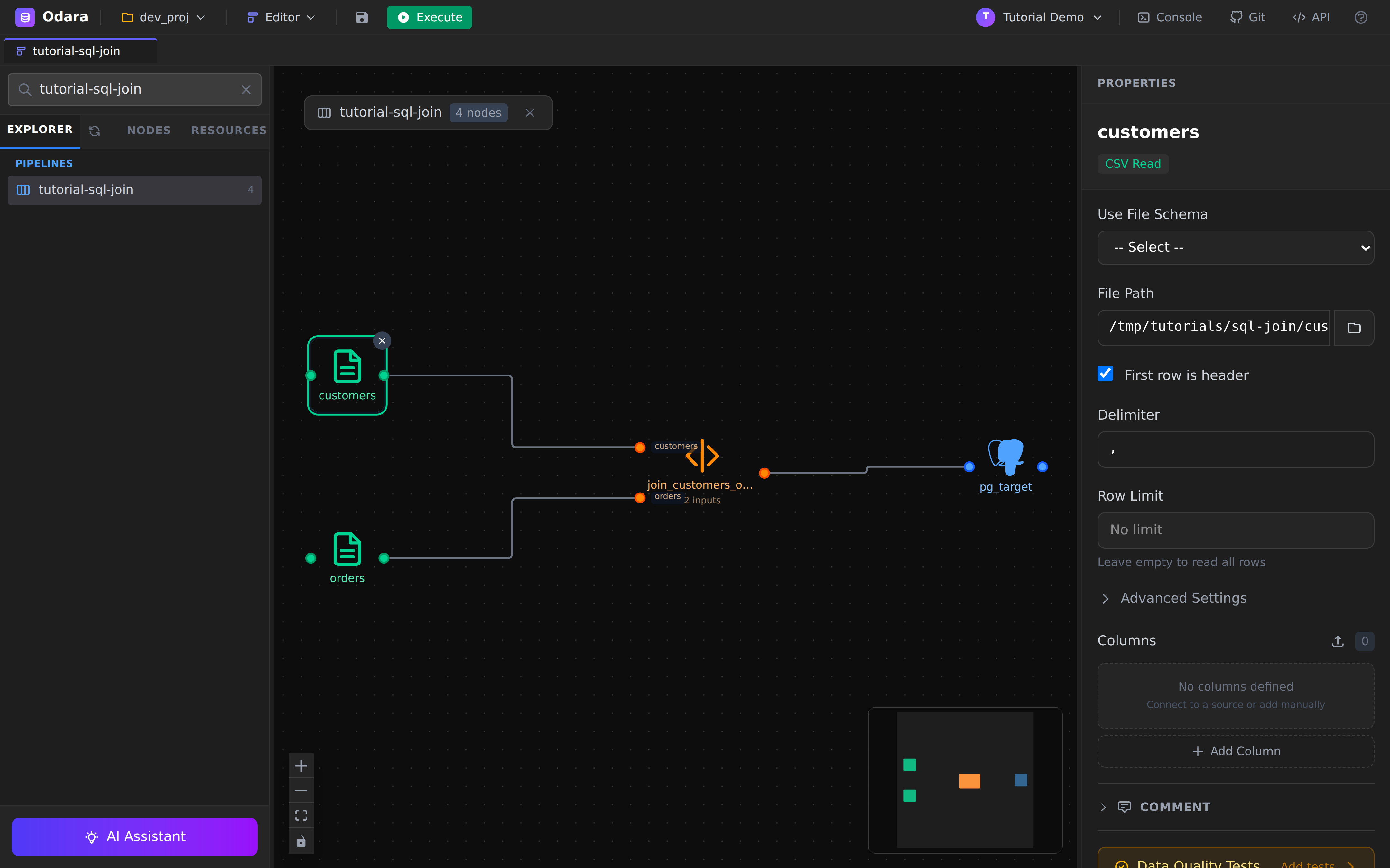
Three things to fill in:
- File Path — absolute path to
customers.csv. Odara reads files from the same machine as the API process, not from your laptop — keep that in mind if the API is running in a container. - Has Header — checked, because the first row of our CSV is column names.
- Delimiter —
,(the default; flip to;or\tif your upstream system likes those).
The schema is inferred on the fly from the file (customer_id,
name, email, country, signup_date) — there's no separate
"declare columns" step.
3. CSV source — orders
Same configuration shape, pointed at orders.csv:
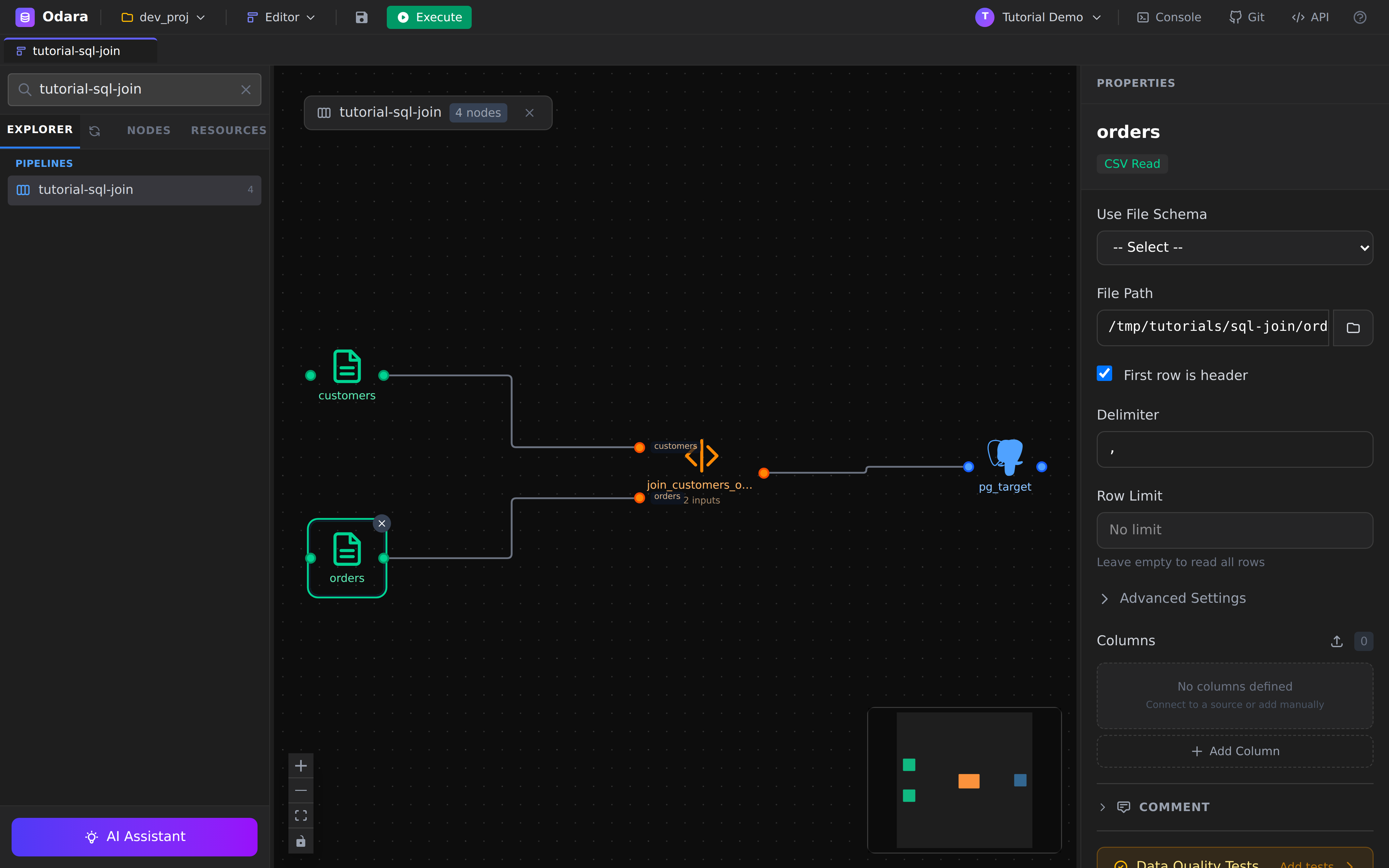
The columns inferred are order_id, customer_id, product,
quantity, total_amount, order_date.
Tip: when you click a source node, the editor offers a Preview Output at the bottom of the Properties panel — handy to confirm the first few rows look right before you wire the downstream nodes.
4. SQL Transform — the JOIN
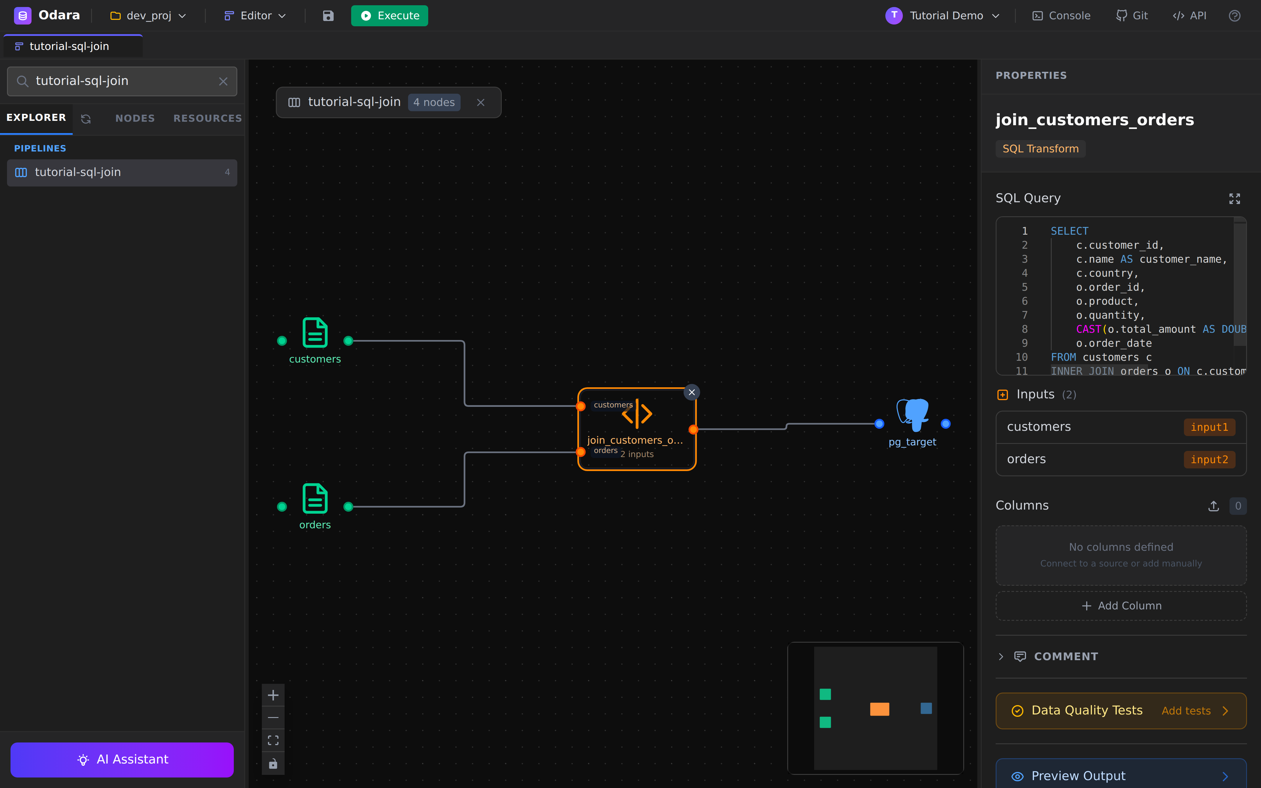
The transform is where the work happens. Click join_customers_orders to see the SQL editor:
SELECT
    c.customer_id,
    c.name AS customer_name,
    c.country,
    o.order_id,
    o.product,
    o.quantity,
    CAST(o.total_amount AS DOUBLE) AS total_amount,
    o.order_date
FROM customers c
INNER JOIN orders o ON c.customer_id = o.customer_id
ORDER BY o.order_date DESC
Three things worth pointing out:
FROM customers candJOIN orders o— these are not the CSV file names. They are the input port names declared on the edges that feed this node. The panel on the right (under Inputs) confirms:customers=input1,orders=input2. Rename the edge labels if you want to read the query with different aliases.CAST(... AS DOUBLE)— Odara uses Arrow types under the hood. The CSV reader returnstotal_amountas a string (since CSV has no types); the cast turns it into a numeric column the Postgres target can write asDOUBLE PRECISION. Without the cast you'd get aVARCHARcolumn on the other side, which works but isn't what you want.No explicit
LIMIT— DataFusion (the SQL engine Odara uses for transforms) is happy to materialise the whole join into a single Arrow batch since the demo dataset is tiny. For real datasets you'd want aWHEREor aLIMITto keep peak memory sane.
5. Postgres Target
Click the rightmost node, pg_target:
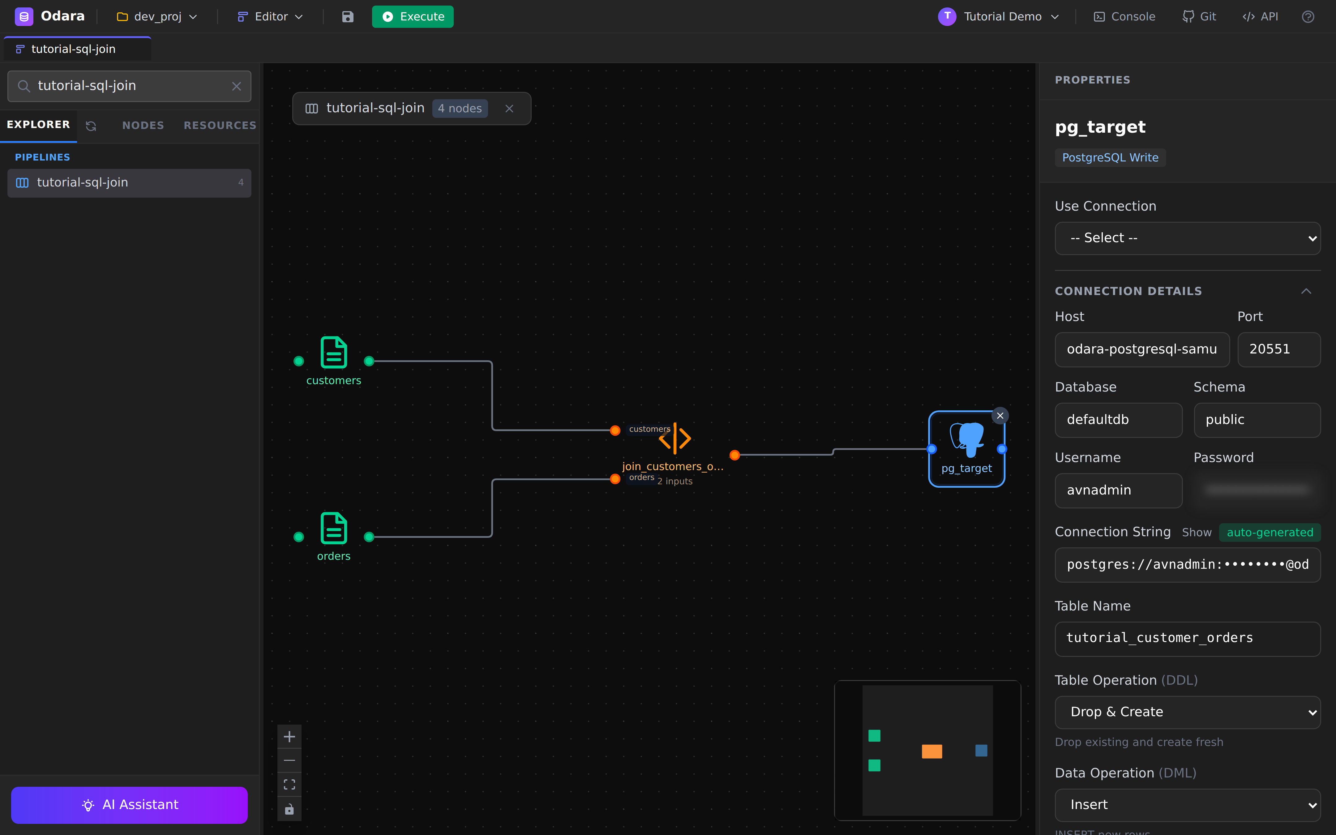
Two ways to wire credentials:
Use Connectiondropdown — pick a previously-saved connection from the project's metadata.- Inline fields — fill
Host,Port,Database,Schema,Username,Passworddirectly. That's what the screenshot above shows (with the password masked).
Either way, the Connection String at the bottom is auto-generated from the structured fields. You can also paste a full connection string and Odara reverses it back into the structured fields — handy for copy-pasting an URL out of your provider's dashboard.
Then four target-shaped fields:
| Field | Value | What it does |
|---|---|---|
| Table Name | tutorial_customer_orders |
Where rows land. The schema (default public) + this name is the fully-qualified target. |
| Table Operation (DDL) | Drop & Create |
Drops the table if it exists, then creates it fresh from the Arrow schema. Re-running the pipeline never accumulates. |
| Data Operation (DML) | Insert |
One INSERT … VALUES (…) batch. For huge datasets see also copy_into on the Snowflake target. |
About
Drop & Create: this is the easiest mode for tutorials and dev work because it makes every run idempotent — you always end with exactly one fresh table. In production you'd usually switch toCreate Table(idempotent at first run, no-op after) orTruncate(preserves indexes/permissions) and route schema changes through migrations, not the pipeline.
6. Execute
The Execute button is in the top toolbar — green when the pipeline is saveable, with a small Stop next to it once a run is in flight.
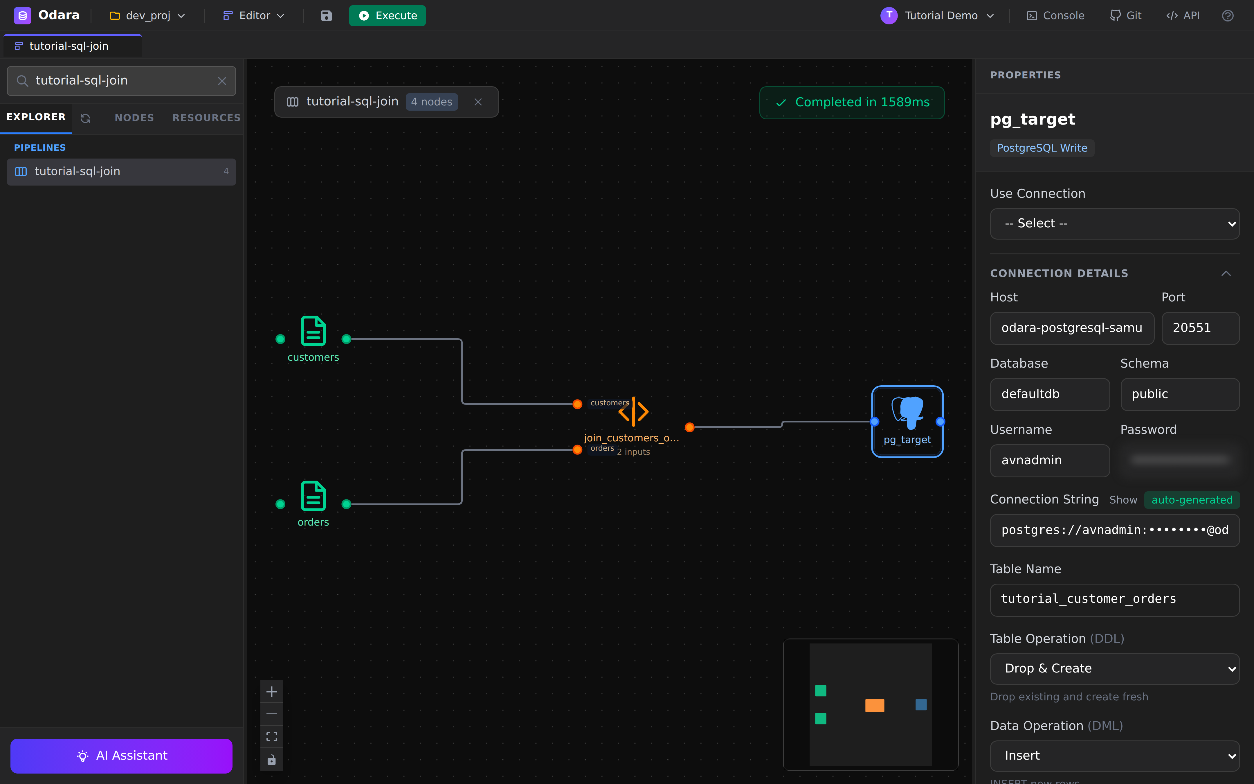
The streaming SSE connection persists every per-node log line to the store, so the trace is also available from Monitor later.
7. Verify in Monitor
Switch to Monitor (top bar Editor ▼ → Monitor) and find the fresh run. It either shows RUNNING for a beat or jumps straight to COMPLETED — the demo dataset takes about a second.
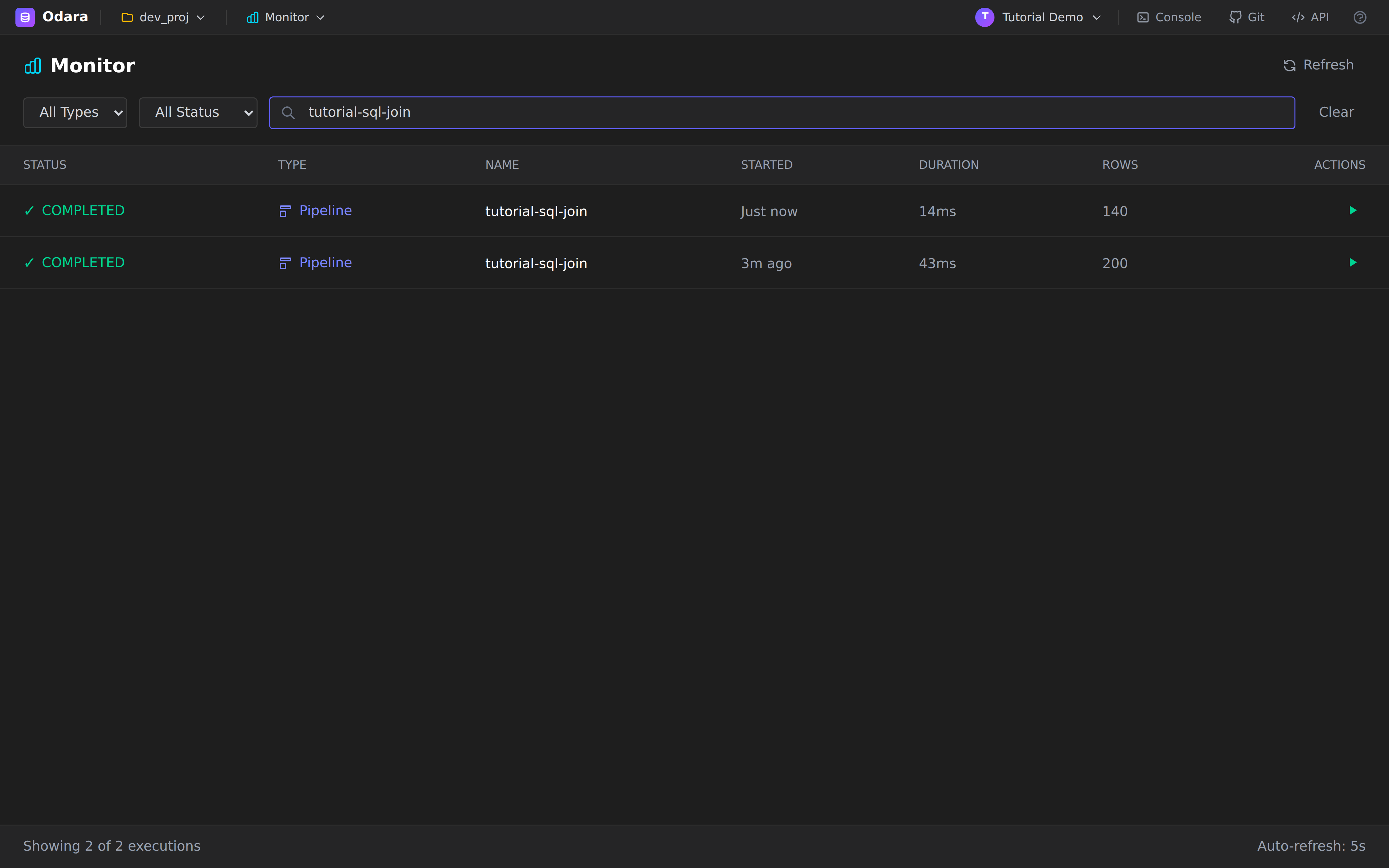
Click the row to open the detail page with the full log trace:
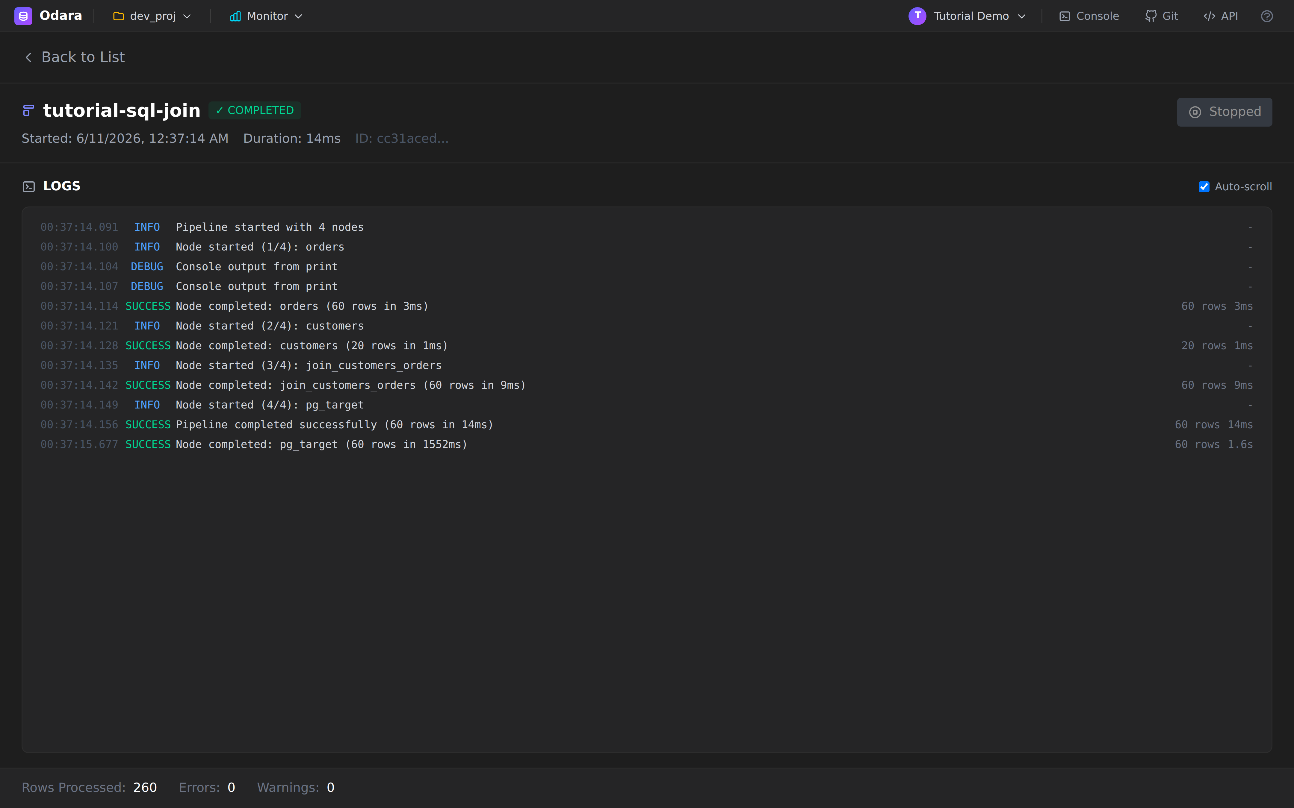
Read the LOGS panel top-to-bottom and you can reconstruct the run:
ordersstarted, finished —60 rows in 3mscustomersstarted, finished —20 rows in 1msjoin_customers_ordersstarted, finished —60 rows in 9mspg_targetstarted, finished —60 rows in 1.6s(network round-trip to the cloud Postgres dominates here)Pipeline completed successfully (60 rows in 14ms)
The Rows Processed: 260 counter at the bottom is the sum of all
nodes' rows: 20 + 60 + 60 + 60 + 60 = 260. Not the number of output
rows — that's 60 (read it off the pg_target line).
8. Verify on Postgres
Open your favourite SQL client (Odara has a Console in the top bar that's a good fit) and run:
SELECT COUNT(*) FROM tutorial_customer_orders;
-- 60

SELECT customer_name, country, product, total_amount, order_date
FROM tutorial_customer_orders
ORDER BY order_date DESC
LIMIT 5;
That returns the same rows that landed at the end of the join, sorted by date.
Cheat sheet
| I want to… | Do this |
|---|---|
| Add a second input to a SQL Transform | Drag a second source onto its left edge — the edge picks up the next free input port name. |
Reference a source as tableX in SQL |
Rename the edge label (input port name), not the source node. |
| Change a CSV's delimiter | Source node → Properties → Delimiter. |
| Re-run without piling up rows | Target node → Table Operation = Drop & Create. |
| Convert a CSV string to a number | CAST(col AS DOUBLE) or CAST(col AS BIGINT) in the SQL Transform. |
| Push to a different schema | Target node → Schema field (default public). |
| See the full log of a finished run | Monitor → click the row → Back to List → click again to force a re-fetch. |
What you learned
- A pipeline can have many sources feeding one SQL Transform — the edge labels become the table aliases in the query.
- Type discipline matters between connectors: cast CSV strings
to a numeric type before the relational target unless you want
VARCHARcolumns on the other side. - The Postgres Target accepts inline credentials or a saved Connection; either way the Connection String at the bottom shows what Odara will actually use.
Drop & Createkeeps tutorial runs idempotent — no leftover rows, no surprise schema drift.
Next
→ Python external + Email — call a .py script and mail the result